Exploring insect wing venation with persistent homology

Code & Notebook on GitHub

This post walks through a Python pipeline for analyzing insect wing venation using persistent homology, a tool from topological data analysis (TDA). By preprocessing wing images into 2D point clouds, we can detect loop structures in the venation using TDA. I demonstrate the method using wing images from a dragonfly, cicada, and grasshopper, and briefly discuss how their structural patterns are shown in persistence diagrams.

Wing photo source: Dragonfly, Cicada, Grasshopper

Procedure

Outline:

• Use scikit-image to preprocess images
• Use scikit-TDA (ripser.py and persim) for topological data analysis

1. Process images

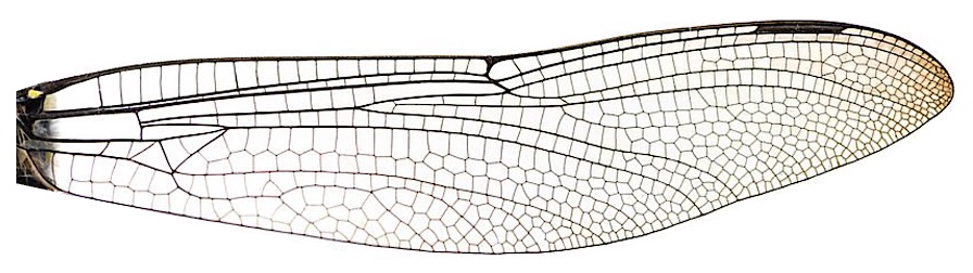
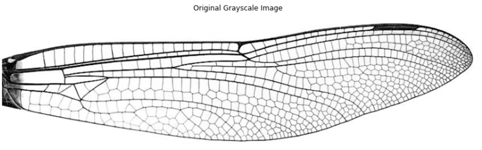
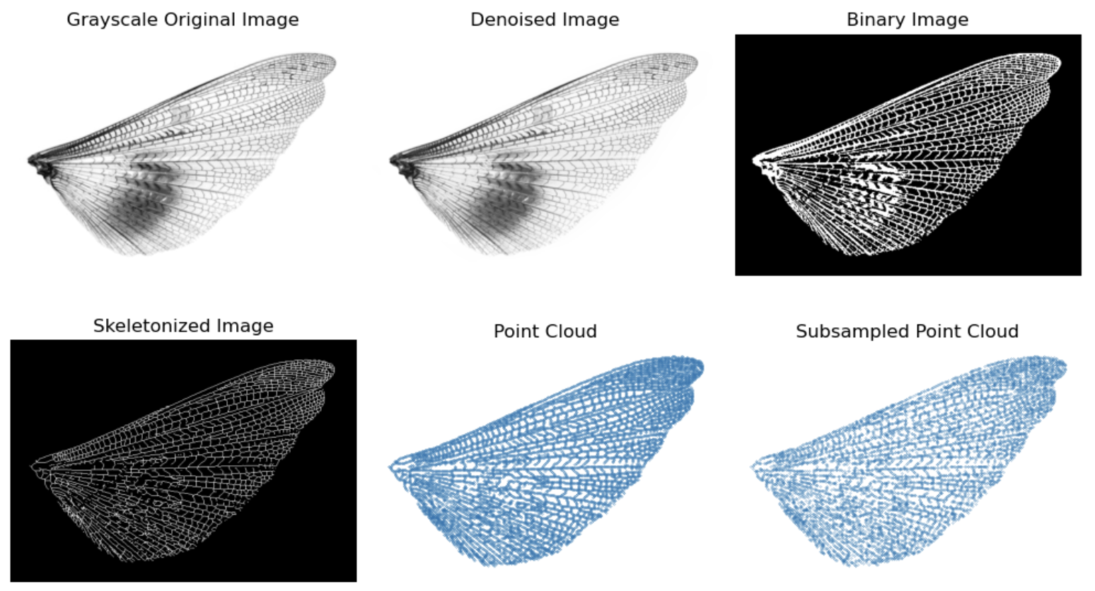
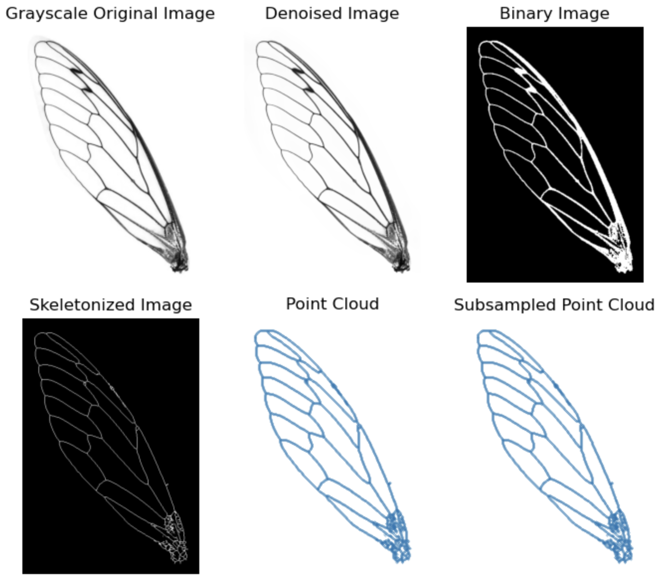
Let’s use a forewing of dragonfly as the example. The image preprocessing includes the following steps:

1. Load image in grayscale
2. Denoise
3. Convert to binary image
4. Skeletonize
5. Make into point cloud

import numpy as np
import matplotlib.pyplot as plt
from skimage import io, color, filters, morphology
from skimage.restoration import denoise_bilateral
from skimage.filters import threshold_local
from skimage.morphology import skeletonize

1.1 Load image in grayscale

img = io.imread("wing_dragonfly.jpg", as_gray=True)

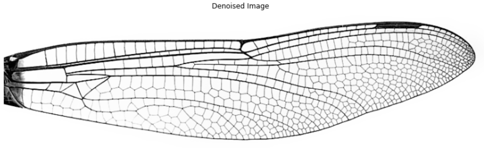
1.2 Denoise

The printed image might not look much different before and after denoising, but it does clean out some dots within the venation windows later in the binary image, which would likely make some difference in TDA results.

img_denoise = denoise_bilateral(img, sigma_color=0.05, sigma_spatial=15)

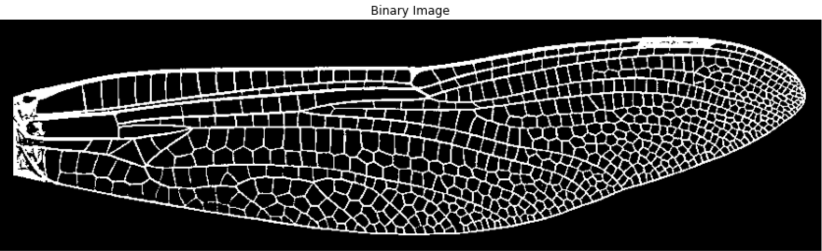
1.3 Convert to binary image

Instead of using a fixed global threshold (which may fail under uneven lighting), we apply local thresholding, which adapts based on the pixel’s neighborhood. The local threshold is computed as the weighted mean of surrounding pixels (set by block_size), minus a constant (offset).

local_thresh = threshold_local(img_denoise, block_size=35, offset=.001)
img_binary = img_denoise < local_thresh

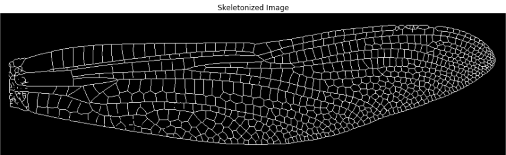
1.4 Skeletonize

Skeletonization reduces each vein to a 1-pixel-wide path, preserving the structure while greatly reducing the number of points.

img_skeleton = skeletonize(img_binary)

1.5 Convert to point cloud

# Get coordinates of all foreground pixels (vein areas)
points = np.column_stack(np.nonzero(img_skeleton))  # shape: (N, 2)

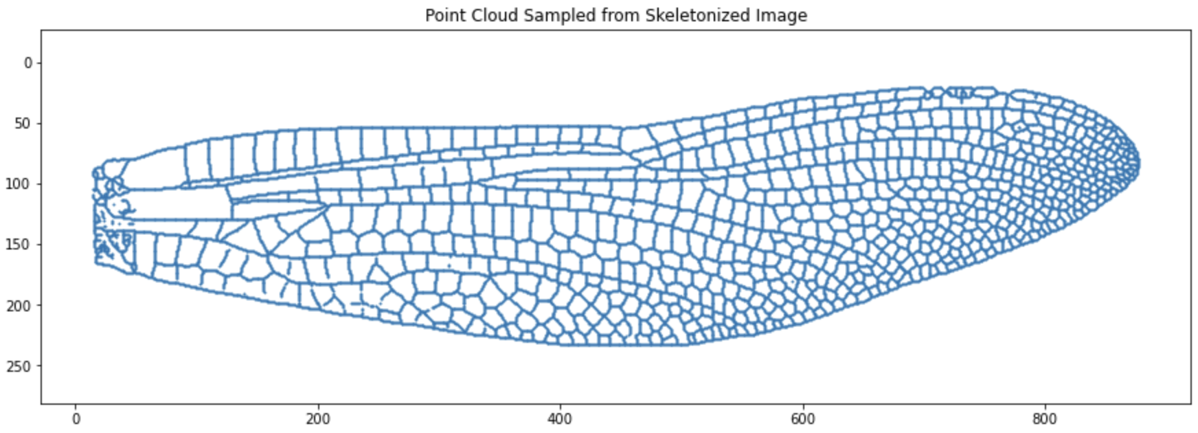
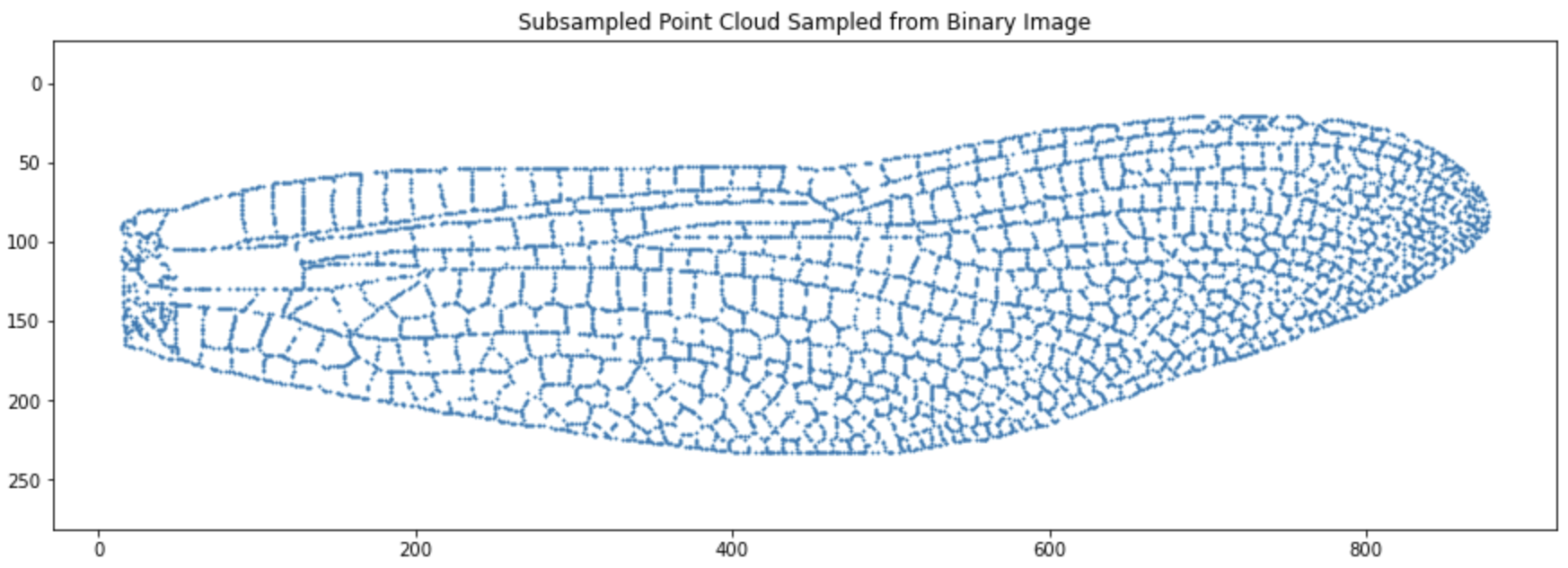
1.6 Subsampling

Subsampling reduces computational cost in TDA, but there’s a trade-off: too few points may miss topological features, while too many increase runtime. Choose n_sample based on dataset size and analysis goals.

idx = np.random.choice(len(points), size=n_sample, replace=False)
points_sampled = points[idx]

2. Topological data analysis (TDA)

We use persistent homology to identify loop-like structures in the wing’s point cloud. Specifically, we apply a Vietoris–Rips filtration to extract H0 (connected components) and H1 (loops). For background, see intro video on TDA by Matthew Wright.

from ripser import ripser
from persim import plot_diagrams

# Rips filtration
result = ripser(points_sampled, maxdim=1)  # setting maxdim=1 would detect H0 and H1 features
diagrams = result["dgms"]

# Plot persistent diagram
plt.figure(figsize=(5, 5))
plot_diagrams(diagrams, show=True, lifetime=True, size=5)

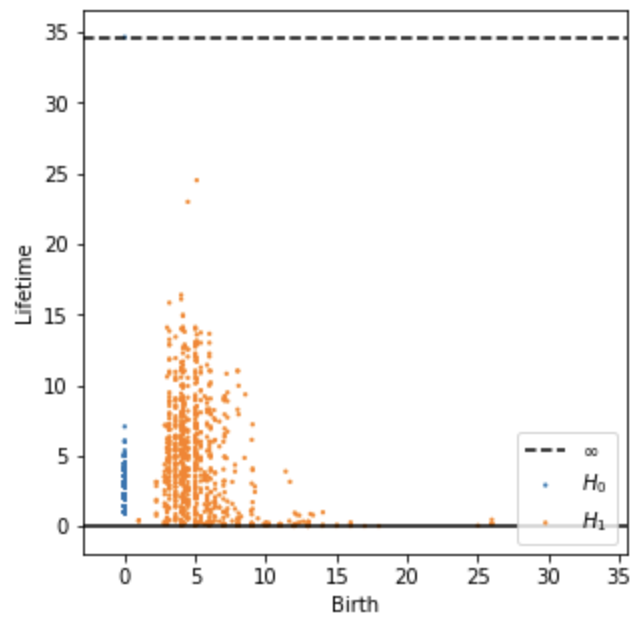
The output persistent diagram shows each detected loops in orange dot (H1), with more “significant” features (those with longer lifespan across distance threshold) locating higher up in y axis, while the less significant or noise features lower down at the bottom. From the results, I suppose the highest two orange points represent the big windows at the top left of the wing.

Applying the workflow to other insect wings

Now I apply the same procedure to process two additional wing images.

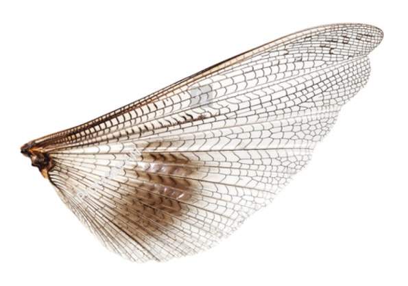
Grasshopper (hindwing)

• Image processing

• Persistence digram

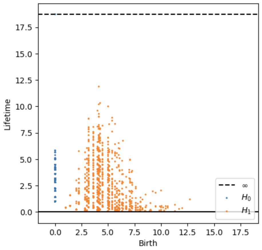
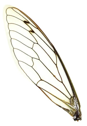
Cicade (forewing)

• Image processing

• Persistence digram

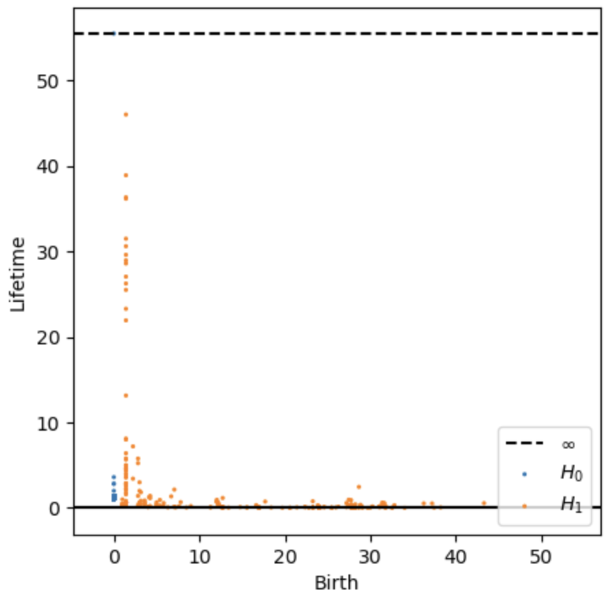
The 15 orange dots higher up in the persistence diagram likely correspond to the 15 distinct windows in the cicada forewing. The dots near the bottom may represent noise or small structures near the wing base.

Refleciton

• Point sampling density significantly affects the persistence diagram, especially the Birth values of H1 features. Choosing the sampling level is a trade-off between computational efficiency and topological fidelity.
  • In densely sampled images (e.g. cicada), true loop structures (wing windows) tend to appear as a vertical line of H1 points with low Birth values but varying Lifetime. Those with higher Birth values are likely to represent noise.
  • In contrast, sparser sampling spreads H1 features more broadly across the birth axis (e.g. grasshopper), making it harder to distinguish true biological structures from noise.
• In this particular case of analyzing wing venation with TDA, the actual venation information is probably mostly captured in the lifetime of H1 features (distribution along the y-axis), whereas the birth axis reflect point sampling density and information about how likely the signals are noise.