Mapping roadkill risk in Taiwan with MaxEnt

Code and data on Github

This note demonstrates how to map roadkill risk in Taiwan using MaxEnt, a presence-only species distribution modeling (SDM) approach. We combine environmental predictors with roadkill occurrences reported by a citizen-science project to estimate a relative risk surface.

This side project was initiated as a submission to the Taiwan Highway Bureau Data Innovative Application Competition, developed in collaboration with Le Quang Tuan and several friends.

Background

The Taiwan Roadkill Observation Network (TRON) has crowd-sourced wildlife-vehicle collision observations since 2011, now accumulated 300,000+ records with species, location, date, and more (a subset of the data is released on GBIF). For a relatively small island, the spatial sampling is dense, offering strong potential for high-resolution risk mapping.

MaxEnt (maximum entropy) works with such presence-only data. It contrasts the environments at presence sites with background samples to estimate a smooth relative suitability surface. Here, instead of speices occurrance for distribution range mapping, we treat roadkill occurrances as presences to model the spatial pattern of relative roadkill risk (focused on the road network).

Workflow

Data sources (all open data)

Occurence data: TRON Roadkill data on GBIF (years 2011-2017, ~46,000 records)
Modeling target: Taiwan highway network (vector)
Environmental predictors:
- Land cover: WorldCover 10 m 2021 v200
- Vegetation: Atlas of Natural Vegetation in Taiwan (not on Github due to file size limit)

I. Prepare data

1. Initialization

Load required libraries

library(terra)
library(sp)
library(dplyr)
library(dismo)

Create raster template

rast <- rast(ext = ext(120, 122.1, 21.8, 25.4), resolution = 0.0009, crs = "EPSG:4326")  # WGS84 CRS

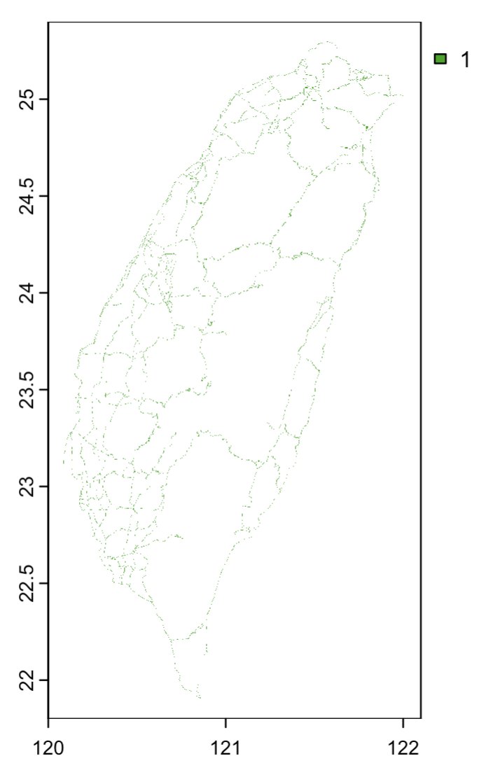
2. Rasterize road data

road.vec <- st_read("data_input/highway/highway.shp") %>%
  st_transform(crs = 4326) %>%
  rasterize(rast, touches = TRUE)
plot(road)

3. Prepare land cover layer

Combine two datasets: vegetation type (for natural vegetation) and WorldCover (for other land types). Vegetation classes take precedence where available.

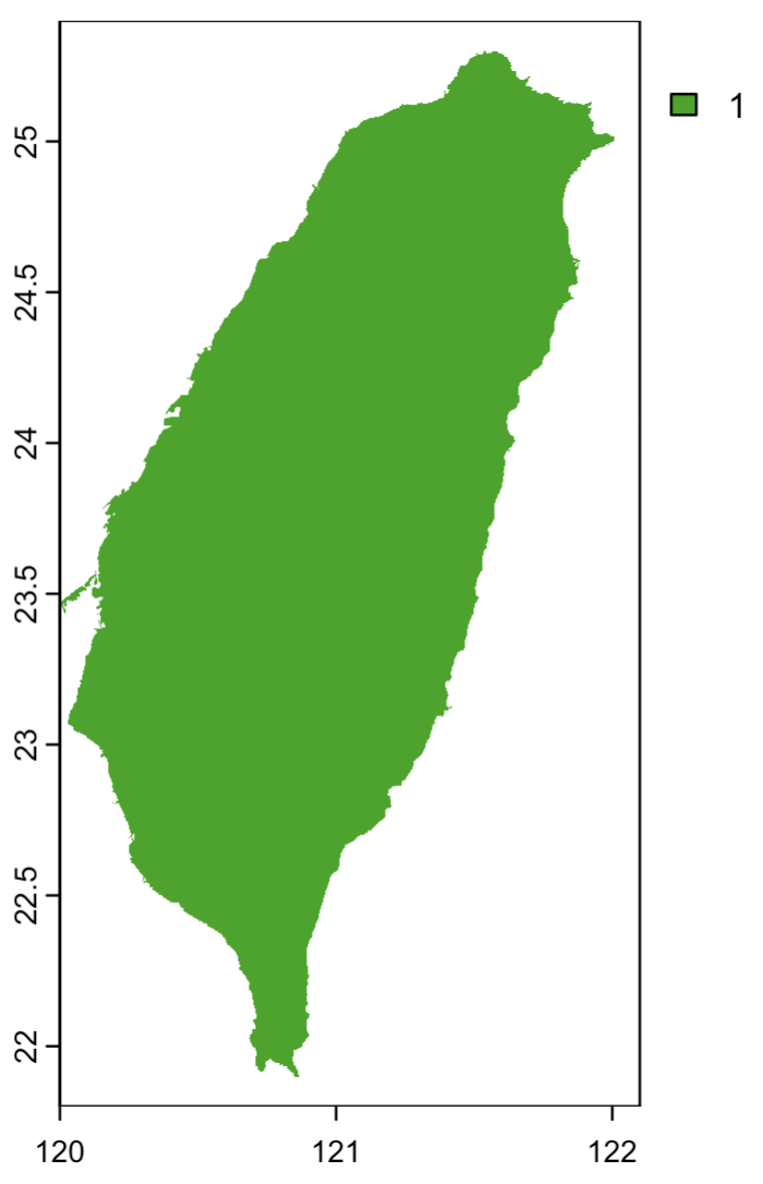
3.1 Create raster of Taiwan island

taiwan.vec <- st_read("data/Taiwan_diss/Taiwan_diss.shp") %>% st_transform(crs = 4326)
taiwan.vec$value <- 1
taiwan <- vect(taiwan.vec) %>% buffer(width = 100) %>%
  rasterize(rast, field = "value", background = NA)
plot(taiwan)

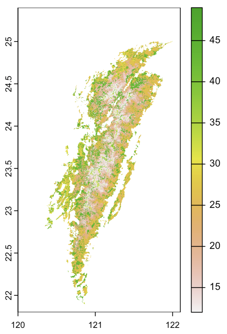
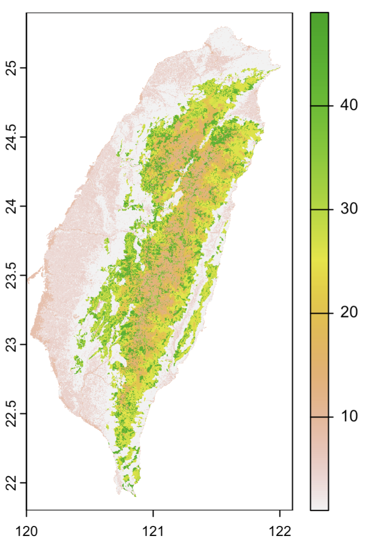
3.2 Process vegetation data (each integer represent a vegetation type)

vegetation.vec <- st_read("data/vegetation/ACO0301000011021.shp") %>% st_transform(crs = 4326)
veg_levels <- unique(vegetation.vec$FORMATION)[c(23,19,10,9,35,17,16,38,20,7,26,37,24,15,
                                                8,4,14,32,5,29,27,18,25,30,28,12,6,33,21,
                                                13,36,1,3,22,2,11,31,34)]
formation_mapping <- setNames(12:(11 + length(veg_levels)), veg_levels)
vegetation.vec$Formation_int <- formation_mapping[vegetation.vec$FORMATION]
vegetation <- rasterize(vegetation.vec, rast, field = "Formation_int", background = NA)
plot(vegetation) # left figure

3.3 Process WorldCover data (each integer represents a land cover type)

worldcover <- merge(rast("data/landcover/ESA_WorldCover_10m_2021_v200_N21E117_Map.tif"),
                    rast("data/landcover/ESA_WorldCover_10m_2021_v200_N21E120_Map.tif"),
                    rast("data/landcover/ESA_WorldCover_10m_2021_v200_N24E120_Map.tif")) %>%
  project(rast, method = "near")
worldcover <- worldcover * taiwan # extract land cover data only within the island
worldcover_mapping <- setNames(1:11,  c(10,20,30,40,50,60,70,80,90,95,100))
values(worldcover) <- worldcover_mapping[as.character(values(worldcover))]
plot(worldcover) # middle figure

3.4 Combine venetation and WorldCover data

unique(c(values(vegetation), values(worldcover)))
land <- worldcover
idx <- which(!is.na(values(vegetation)))
values(land)[idx] <- values(vegetation)[idx]
plot(land) # right figure
writeRaster(land, "data/land.tif")

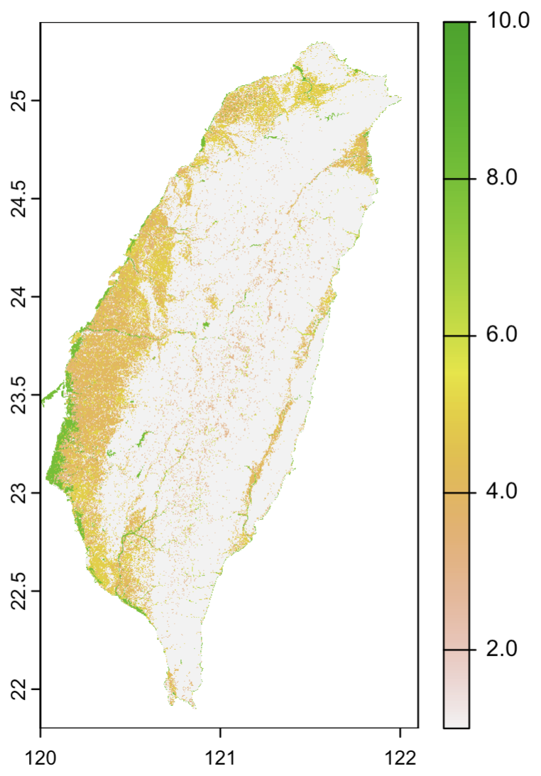
(rendered in continuous color palette, but these are caterogical data)

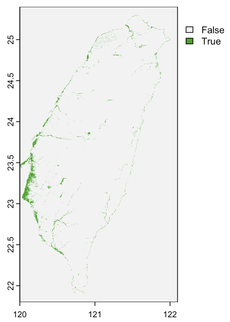
4. Create “distance to water” layer

Compute distance to water (only for the road cells to save computation time)

water <- land == 8
plot(water)
values(water)[which(is.na(values(water)))] <- FALSE

roadwater <- water
values(roadwater)[which(values(road) == 1)] <- NA
dist_to_water <- distance(roadwater, target = NA, exclude = FALSE)
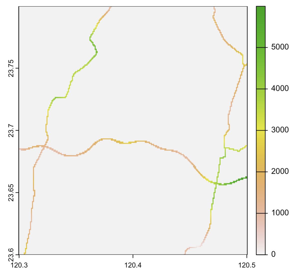
# plot(dist_to_water)
plot(crop(dist_to_water, ext(120.3, 120.5, 23.6, 23.8))) # zoom in

writeRaster(dist_to_water, "data/dist_to_water.tif")

II. Build model

1. Load required libraries

MaxEnt is implemented in Java but can be called in R through package susch as dismo (used here). You’ll need to download “maxent.jar” from the Maxent website and place it where dismo expect it. There are other Jave-free R packages implementing Maxent models, such as maxnet (workflows via package ENMeval).

library(dplyr)
library(raster)
library(dismo)
library(rJava)

2. Load predictors (rasters)

# load data
road <- raster("data/road.tif")
pred.dWater <- raster("data/dist_to_water.tif")
pred.land <- raster("data/landcover.tif")

# keep only grid cells on road
pred <- stack(pred.land, pred.dWater) %>% mask(road)
names(pred) <- c("landcover", "dis_to_water")

3. Load occurance data (roadkill records)

Different taxa may respond differently to the same predictors due to different habitat preference or behaviors, so it may be better to model different groups separately. Here I’m using amphibians and reptiles (herpets) as example.

# load data
rk_herpet_raw <- read.csv("data_input/roadkill.csv") %>%
  filter(class %in% c("Squamata", "Amphibia")) %>%
  rename(lon = decimalLongitude, lat = decimalLatitude) %>%
  select(lon, lat)

# keep only points that fall on valid predictor cells
on_target <- apply(!is.na(extract(pred, rk_herpet_raw)), 1, all)
rk_herpet <- rk_herpet_raw[on_target, ]

4. Fit MaxEnt model and make prediction

set.seed(123)
m.herpet <- maxent(x = pred,
                   p = rk_herpet,
                   nbg = 100000,
                   factors = "landcover",
                   removeDuplicates = FALSE)
m.herpet # show summary (open as an HTML page)

x: spatial object of predictor layers
factors: specify which predictor layers are categorical
p: occurence data (roadkill records) in coordinates
nbg: number of background points
By default, duplicate presences within a cell are removed to reduce sampling bias; override with removeDuplicates = FALSE.

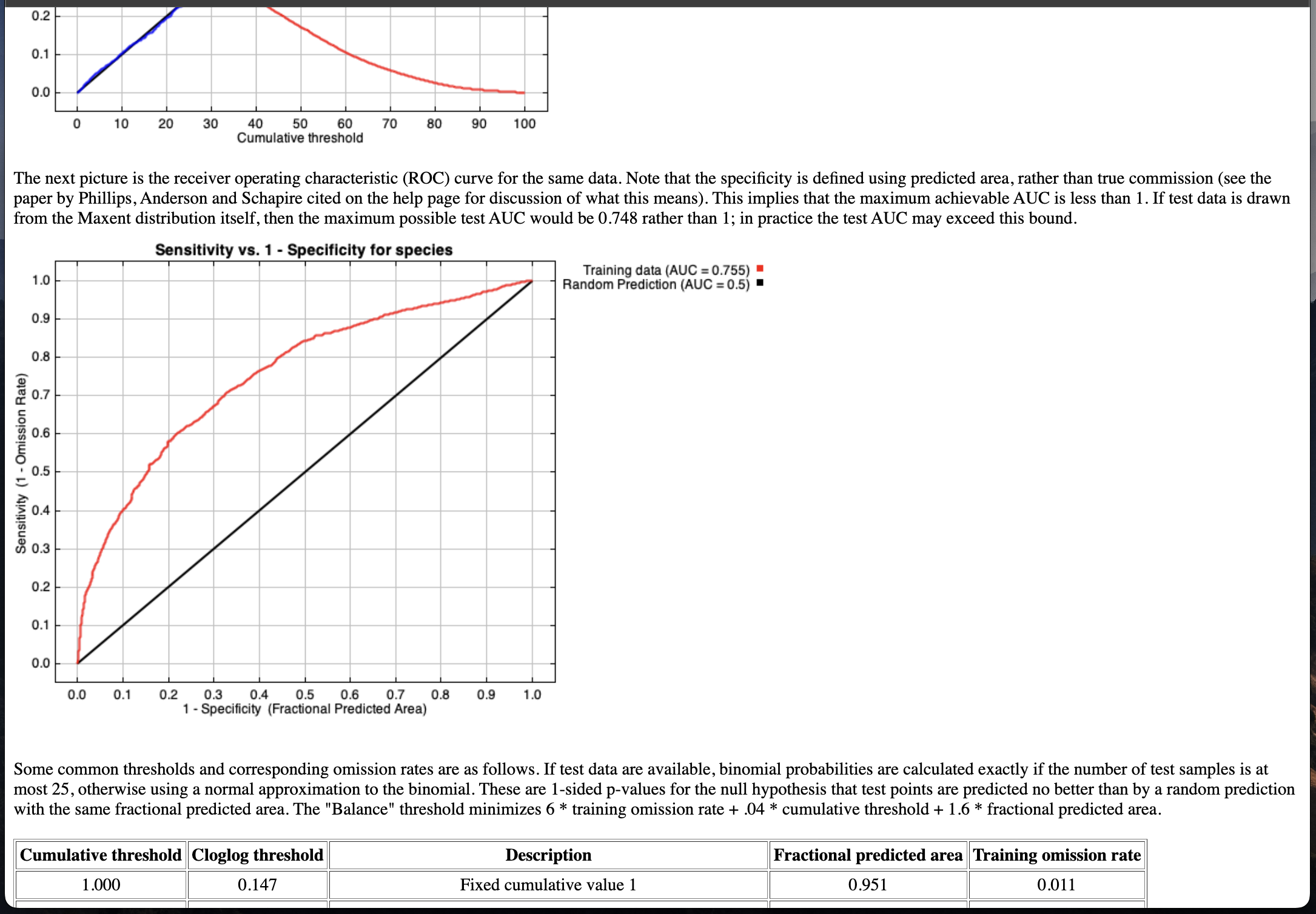
The HTML summary includes model AUC, variable contributions, threshold-based diagnostics, etc.

# Check fitted response
response(m.herpet)

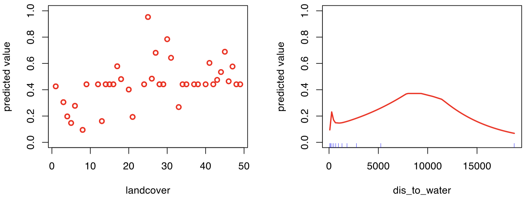
The left plot shows the categorical land-cover effect (here displayed as integer codes because labels were mapped to integers). We can retreive the labels to gain insight into their effects, but I’m skipping this step since this is just a demonstration.

The right shows the continuous effect of distance to water (in meters). Let’s focus on ~0–1 km, where risk increases as roads get closer to water, which makes sense for amphibians and reptiles. At zero, the risk drops sharply likely because many near zero distance are bridges (road over water), where terrestrial animals are relatively rare. Beyong a few kilometers, effects are probably less meaningful and may reflect data sparsity rather than true patterns.

# Predict roadkill risk
risk <- predict(pred, m.herpet)
plot(risk)

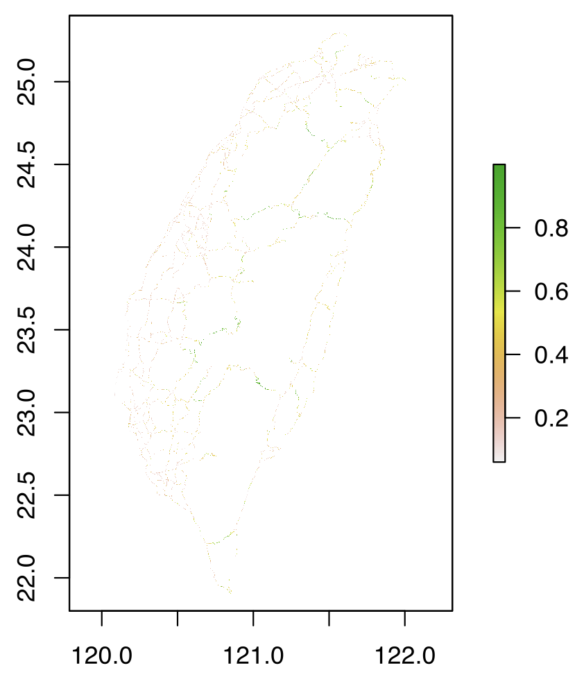
You can see that such plot makes roads look nearly invisible at island scale (narrow linework). So in the next part, we are gonna make some efforts to better visualize the result.

III. Visualize risk predictions

Now let’s create interactive maps that allow zooming for details. We can also add the roadkill records onto the map to provide more background information.

Load required libraries

library(sf)
library(mapview) # interactive map

Interactive map + presence points (raster)

rk_points <- st_as_sf(rk_herpet, coords = c("lon", "lat"), crs = 4326)

mapviewOptions(basemaps = c("CartoDB.DarkMatter", "OpenStreetMap", "Esri.WorldImagery", "OpenTopoMap"))
mapview(risk, maxpixels = 9332000, layer.name = "Roadkill risk", na.color = "transparent") +
  mapview(rk_points, layer.name = "Roadkill records (herpet)", cex = 5, alpha = .1, col.regions = "white")

In case the embedded html does not load, you should see a zoomable map like this:

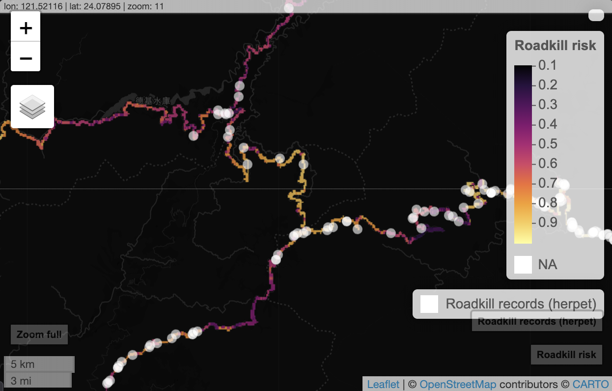
This is now better. But because rasters render as thin lines for roads, they remain hard to see at small scales. To improve readability, we convert the information into vectors (sample along road vectors and visualize smoothed segment values).

Interactive map + presence points (vector)

# create road vector
road.vec <- st_read("data_input/highway/highway.shp") %>% st_transform(st_crs(risk))

get_smooth_vect <- function(risk) {
  # extract risk values along road vectors (at vertices) from risk raster
  coords <- st_coordinates(road.vec)
  risk.points <- extract(risk, coords[, c("X", "Y")])

  # compute risk values of segments (midpoint average between consecutive vertices)
  risk.seg <- (risk.points[-length(risk.points)] + risk.points[-1]) / 2
  valid <- (coords[-nrow(coords), "L1"] == coords[-1, "L1"]) &
    (coords[-nrow(coords), "L2"] == coords[-1, "L2"])
  risk.seg <- risk.seg[valid]

  # create line segments
  coords_from <- coords[-nrow(coords), ][valid, ]
  coords_to <- coords[-1, ][valid, ]
  segments <- lapply(seq_along(risk.seg), function(i) {
    st_linestring(rbind(coords_from[i, c("X", "Y")], coords_to[i, c("X", "Y")]))
  })

  # compute moving average
  moving_average <- function(values, window) stats::filter(values, rep(1 / window, window), sides = 2) %>% as.numeric
  risk.seg.smooth <- moving_average(risk.seg, window = 100)
  risk.seg.smooth[is.na(risk.seg.smooth)] <- risk.seg[is.na(risk.seg.smooth)]

  # return sf object
  risk_smooth_sf <- st_sf(geometry = st_sfc(segments, crs = st_crs(road.vec)),
                          mean_value = risk.seg.smooth)
  return(risk_smooth_sf)
}

risk_smooth_herpet <- get_smooth_vect(predict(pred, m.herpet))

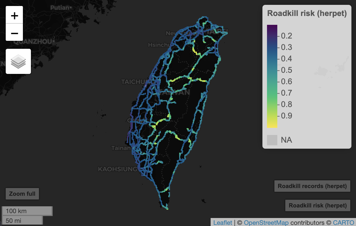
mapview(risk_smooth_herpet, zcol = "mean_value", layer.name = "Roadkill risk (herpet)") +
  mapview(rk_points, layer.name = "Roadkill records (herpet)", cex = 5, col.regions = "white")

Now you can see the roadkill risk along highways across Taiwan. You can toggle off the roadkill records (from top left layer icon) to remove points blocking the view.

If page doesn’t load, the expected view looks like this:

Remarks

Practical implications

This is just a quick prototype, so I don’t want to overinterpret the results. But with more careful model design, tuning, and bias handling, this kind of model can have practical implications for conservation:

Hotspot prioritization: The risk map can be used to flag road segments that warrent attention and could be targeted for preventive measures (fencing, speed reduction, animal passage, etc.).
Clues about causes: The fitted response indicates the environmental factors correlated to risk, which help form hypotheses about animal movement and humand-wildlife interaction.

How this differs from classic SDM

Traditional SDMs treat presences as places a species can persist. In roadkill risk, a “presence” is a collision event—the outcome of species occurrence × movement/crossing behavior × road design/traffic × reporting effort. Because of that, some common SDM practices may need to be adapted to this specific context. Below includes a few exmaples.

Caveats and future directions

Background bias: The default background points were sampled uniformly along roads, but reporting effort isn’t uniform—busy and accessible roads are likely reported more. A potential correction is “target-group background”, where we can draw background from all roadkill submissions to approximate reporting effort (i.e. contrasting the focal taxa with all species)—as in Chyn et al. (2021). However, because roadkill frequency can also reflect true risk, this may absorb some signal. An alternative may be to weight background by other effort proxy (such as traffic volumn) to better reflects where people and vehicles actually are.
Duplicates records: By default, Maxent keep one occurance record per cell to account for effort bias. But for roadkill, multiple records might reflect genuine risk signal (not just effort). Keeping all records might make sense if we can have an effort weighted background.
Overfitting issue: Split train/test sets by space (and by time if possible) can give more honest output than random splits (especially in clustered data) to help avoid overfitting.
Scope of this demo: I’m using a small subset of roadkill data, highway only, and just two predictors, for demonstration. Data exists for more in-depth exploration.