Phylogenetic tree with trait mapping
==
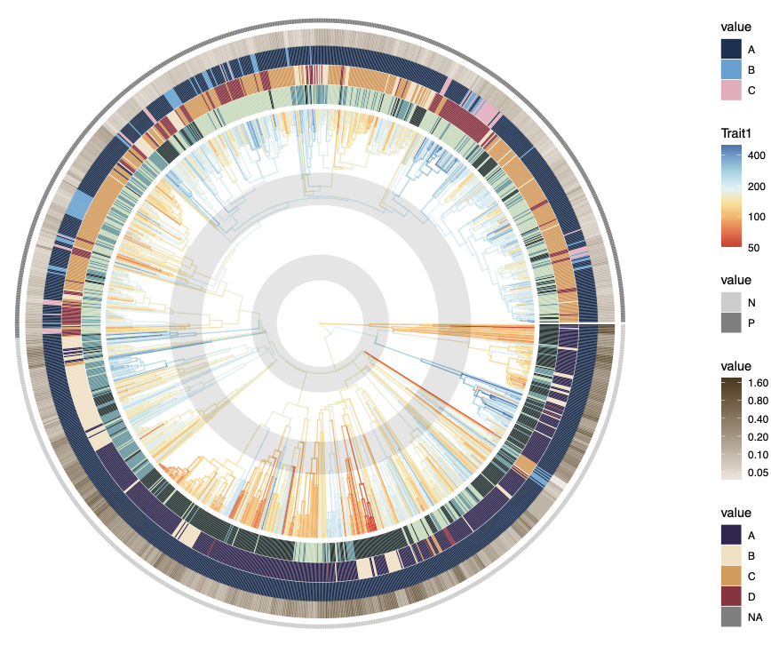
This note demonstrates how to visualize a phylogenetic tree with species-level trait data using R (the workflow behind Figure 4 in Hung et al. 2022). The tree can be plotted in either circular or linear layout formats:
1. Prepare data
1.1 Required libraries
library(ggtree)
library(phytools)
library(ggplot2)
library(ggnewscale)
1.2 Required datasets
- A phylogenetic tree object (
tree) in .tre format - A species-trait dataset (
trait) with species names matching the tree’s tip labels
1.3 Clean data
Reorder the trait table to match the order of species in the tree:
is_tip <- tree$edge[, 2] <= length(tree$tip.label)
ordered_tips <- tree$edge[is_tip, 2]
trait <- trait[match(tree$tip.label[ordered_tips], trait$Species), ]
Set row names to species names for downstream compatibility:
rownames(trait) <- trait$Species
Example of cleaned-up species-trait data. Traits can be either continuous or categorical.
| (rowname) | Taxonomic group | Trait 1 | Trait 2 | Trait 3 | Trait 4 | Trait 5 |
|---|---|---|---|---|---|---|
| Scientific_name_1 | A | 428 | A | C | A | 0.09 |
| Scientific_name_2 | A | 274 | C | D | B | 0.08 |
| Scientific_name_3 | B | 331 | C | C | B | 0.24 |
| Scientific_name_4 | B | 189 | A | B | C | 0.11 |
| … | … | … | … | … | … | … |
In this tutorial, We’ll map:
- Trait 1 to tree branch color
- Traits 2–5 to concentric rings (using
gheatmap) - Group to the outermost thin ring
1.4 (Optional) Estimate ancestral state
If we want to color the tree using ancestral trait values, we’ll need to reconstruct internal node states. Otherwise, we can plot a single colored tree and skip this part.
1.4.1 Estimate node values
For demonstration, I use phytools::fastAnc() to estimate ancestral node values for a continuous trait (Trait 1). Depending on the size of the dataset, this step could be very computationally intensive.
There are a lot of tools for ancestral state reconstruction based on specific assumptions and data format. If we already have the estimated data, just import it (and sort out how to match the data format).
trait.1 <- trait$Trait1
names(trait.1) <- rownames(trait)
fit <- fastAnc(tree, trait.1) # computationally intensive
# fit <- readRDS("ans_fit.rds") # or import fitted data
1.4.2 Merge node values into the tree data
tip_data <- data.frame(node = nodeid(tree, names(trait.1)), Trait1 = trait.1)
node_data <- data.frame(node = as.numeric(names(fit)), Trait1 = as.numeric(fit))
data <- rbind(tip_data, node_data)
tree <- dplyr::full_join(tree, data, by = "node")
2. Plotting the tree
2.1 Basic Tree with Trait 1 Coloring
Let’s first try out the default setting (omit aes(color = Trait1) if not plotting ancestral values).
ptree <- ggtree(tree.plot, aes(color = Trait1), layout = "circular", ladderize = F)
print(ptree)
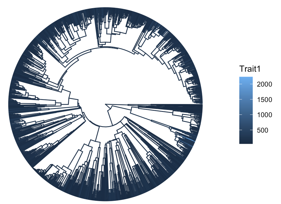
The default color scale may not reflect the full variation in Trait 1. Let’s customize the color scale for better contrast:
palette1 <- RColorBrewer::brewer.pal(n = 8, name = "RdYlBu")
colors1 <- colorRampPalette(palette1)(100)

ptree <- ggtree(tree.plot, aes(color = Trait1), layout = "circular", ladderize = F) +
  scale_colour_gradientn(colors = colors1, trans = "log", limits = c(50, 500),
                         breaks = c(50, 100, 200, 400), oob = scales::squish) +
  annotate("rect", xmin = 22, xmax = 35, ymin = -Inf, ymax = Inf, alpha = .1, fill = "black") +
  annotate("rect", xmin = 60, xmax = 76.5, ymin = -Inf, ymax = Inf, alpha = .1, fill = "black")

print(ptree)
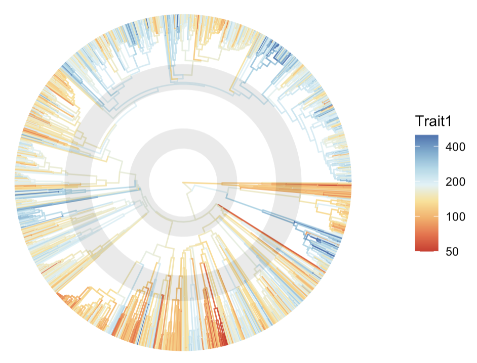
Key elements explained:
-
trans = "log": fit the right-skewed data distribution on the color scale -
"limits = c(min, max)": cap the lower and upper limit of the color scale (to manage outliers) -
oob = scales::squish: squish extreme values into the limits (e.g. an outlier of 1,000 will be shown in the same color as 500, which is the max) -
breaks: specify the ticks on the legend
A red-yellow-blue color ramp is employed using the following functions:
-
RColorBrewer::brewer.pal(): create color palette (a vector of several colors) -
colorRampPalette(): extend that color palette to a ramp of 100 colors
I also add two rings that highlight the time period of interest (in this example, the adaptive radiation events in modern bird evolution) using annotation().
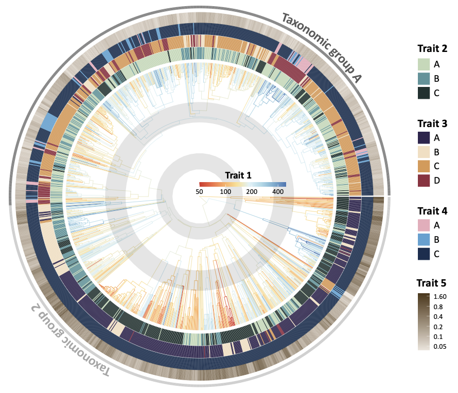
2.2 Add triat rings with gheatmap()
# trait 2 (categorical)
p <- gheatmap(ptree, trait[, "Trait2", drop = F], width = 0.09, offset = -2, color = NULL, font.size = 0) +
  scale_fill_manual(values = c(A = "#203331", B = "#55949A", C = "#C1D9B7"))

# trait 3 (categorical)
p <- p + new_scale_fill()
p <- gheatmap(p, trait[, "Trait3", drop = F], width = 0.09, offset = 8, color = NULL, font.size = 0) +
  scale_fill_manual(values = c(A = "#302650", B = "#F3DEC0", C = "#DC9750", D = "#922C40"))

# trait 4 (categorical)
p <- p + new_scale_fill()
p <- gheatmap(p, trait[, "Trait4", drop = F], width = 0.09, offset = 18, color = NULL, font.size = 0) +
  scale_fill_manual(values = c(A = "#173050", B = "#54A2D2", C = "#EBAABB"))

# trait 5 (continuous)
p <- p + new_scale_fill()
p <- gheatmap(p, trait[, "Trait5", drop = F], width = 0.08, offset = 28, color = NULL, font.size = 0) +
  scale_fill_gradient(low = "#ede6dd", high = "#4d3718", trans = "log", breaks = c(.05, .1, .2, .4, .8, 1.6))

# taxonomic group (outer thin ring)
p <- p + new_scale_fill()
p <- gheatmap(p, trait[, "Group", drop = F], width = 0.02, offset = 43, color = NULL, font.size = 0) +
  scale_fill_manual(values = c(P = "gray50", N = "gray80"))

print(p)
Key elements explained:
-
scale_fill_manual(values = c(A = colorA, B = colorB, C = colorC)): manually assign colors to each trait values. Name the color values (colorA, …) with the trait values (A, …) in the vector. -
width: specify the width of the ring -
offset: adjust the distance of the ring from the central tree -
font.size = 0: avoid showing labels -
ggnewscale::new_scale_fill(): This is required to add a new ring with a different color scheme
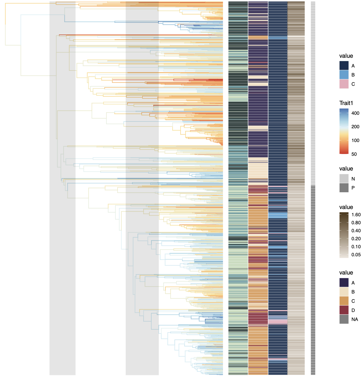
[Alternative] Linear layout option
To switch to a traditional linear tree layout, just omit layout = "circular":
3. Final Touches
I often export the tree and customize the legend and annotations in PowerPoint for clarity:
We can also add silhouettes or icons to tips for visual taxonomy. Check out PhyloPic for public domain silhouette images.