Pairwise beta diversity tutorial

Note: This material was created for leading the discussion in the course Frontiers in Biodiversity Measurement (Fall 2021) at the University of Maryland.

Main reference: Marion et al. (2017) Pairwise beta diversity resolves an underappreciated source of confusion in calculating species turnover.
Data source for R tutorial: Harrison et al. (2018) Phylogenetic homogenization of bee communities across ecoregions.

Background

Beta Diversity

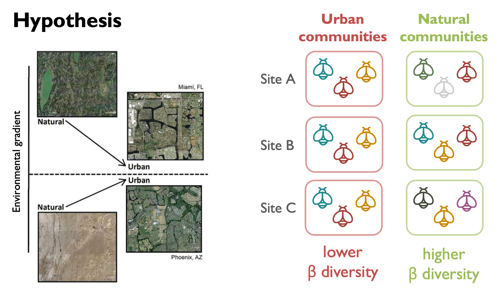
Beta diversity is the degree of differentiation among biological communities.

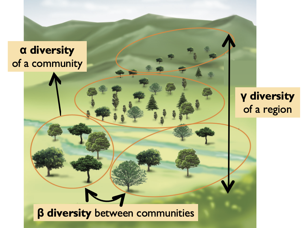
Image adapted from Tamilnadu Board 12th Class Biology textbook

Say $\alpha$ is the species diversity of a community, and $\gamma$ is the total species diversity of a region composed of multiple communities. For a system with $N$ communities, Beta Diversity can be defined as $\beta = \gamma/\alpha$ (Whittaker 1960).

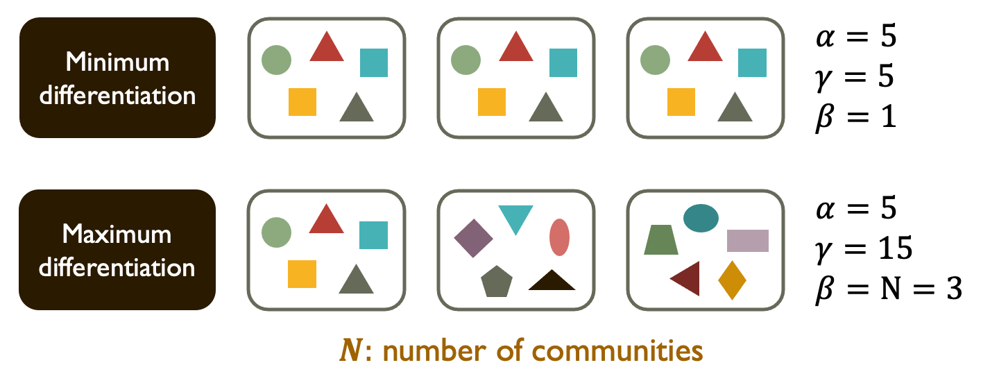
However, as $\beta$ can range from $1$ to $N$, this measure is not comparable between systems with different $N$.

Turnover Rate

Turnover Rate provides a more standardized measure, defined as $T=\dfrac{\beta-1}{N-1}$ where $T$ ranges from 0 to 1. However, this measure is sensitive to sample size. Let’s look at the following example.

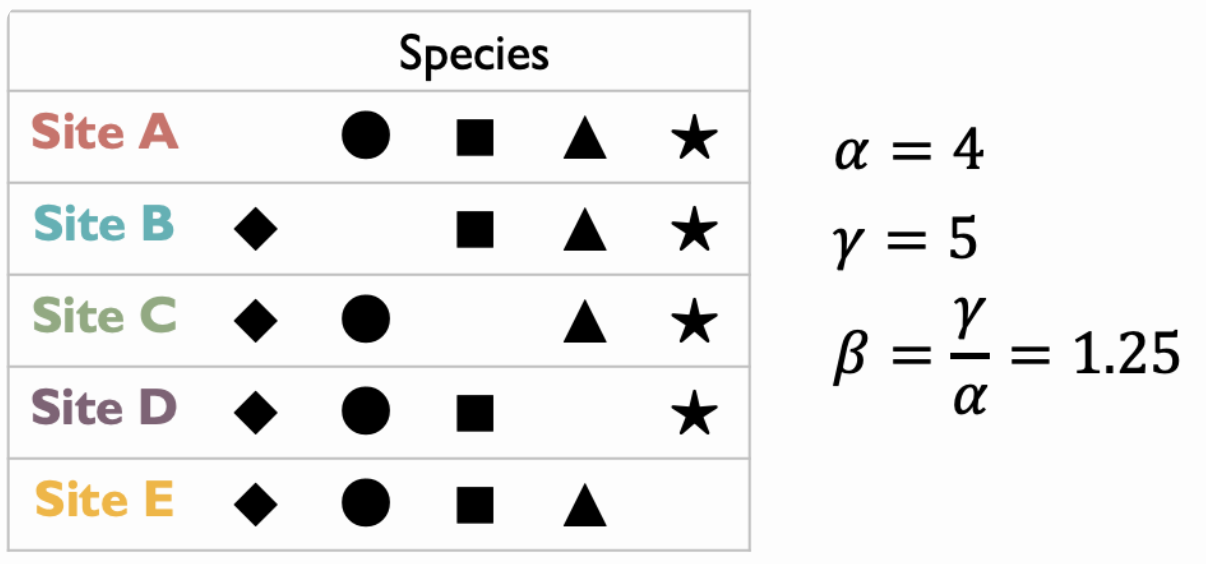
In this system with 5 communities, if we have a complete sample of all sites:

\[N=5,\ \ T=\dfrac{\beta-1}{N-1}=\dfrac{1.25-1}{5-1}=\dfrac{1}{16}\]

For incomplete sampling, $T$ can be overestimated:

\[N=4,\ \ T=\dfrac{1.25-1}{4-1}=\dfrac{1}{12}\] \[N=3,\ \ T=\dfrac{1.25-1}{3-1}=\dfrac{1}{8}\] \[N=2,\ \ T=\dfrac{1.25-1}{2-1}=\dfrac{1}{4}\]

Pairwise Dissimilarily

In order to resolve these problems, Marion et al. (2017) introduced pairwise beta diversity as a unbiased measure of species turnover. This is done by computing the turnover rate for every community pair, and then take the average.

Let’s look at the same example as the above, with 5 communities in the system. Every community pair ($N=2$) has a turnover rate: $N=2,\ \ T=\dfrac{1.25-1}{2-1}=\dfrac{1}{4}$

And then we compute the average of the observed turnover rates $\bar{T}$, which is 1/4. Even when we only sample part of the communities, the measure remains unchanged.

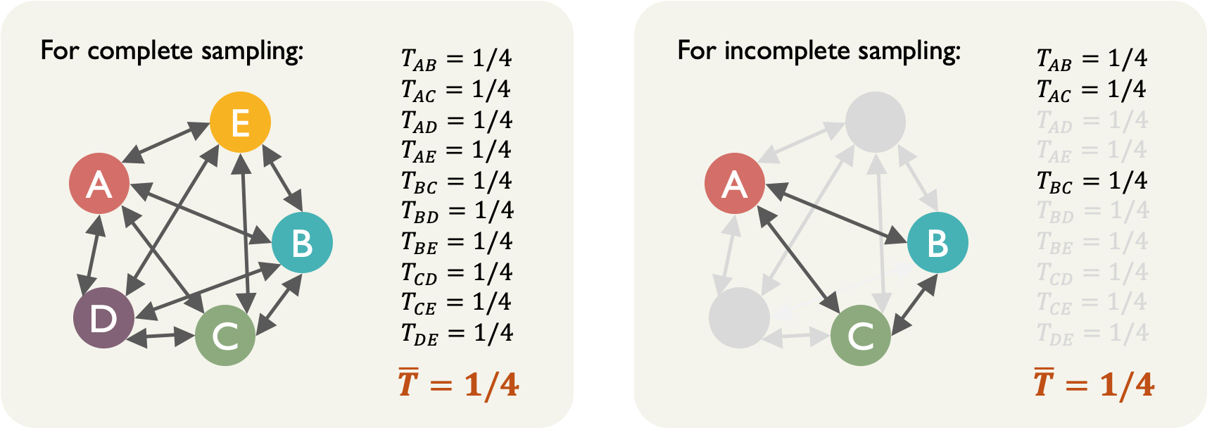
An intuitive understanding of this measure $\bar{T}=1/4$ is “one out the four species present within a site is not expected to be present in a second site”.

R tutorial: A comparison between N-community and mean pairwise dissimilarity beta diversity measures

You want to know whether urbanization can lead to ecological homogenization in bee communities. In other words: are bee communities in urban habitats more similar to each other than communities in forests or agricultural lands?

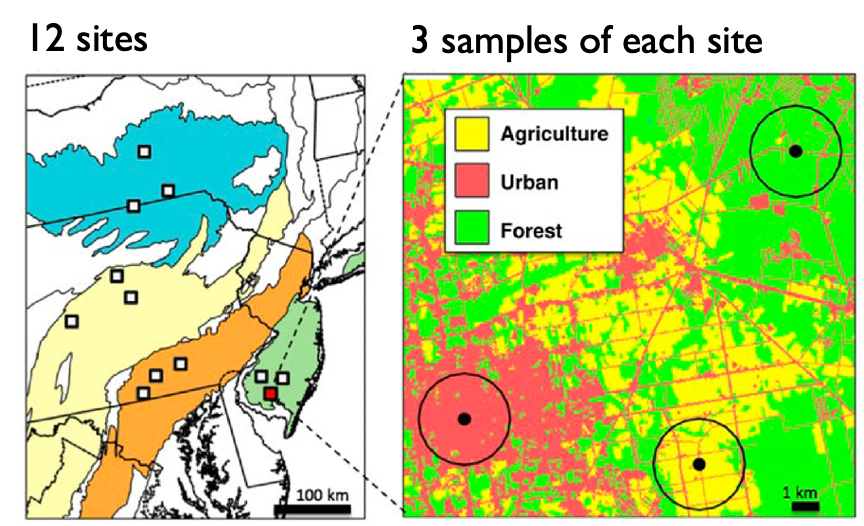
You plan to collect samples from 12 sites, each with three habitats: agricultural, forest, and urban. That makes 36 community samples in total.

library(ggmap)
library(ggplot2)

# these are the locations of the blocks
site <- read.csv("site_data.csv") # import sampling site data

# take a look at where the 36 locations are
map <- get_stamenmap(bbox = c(left=-78.6, bottom=38.6, right=-73.2, top=43), zoom=7)
ggmap(map) + geom_point(site, mapping = aes(x=lon, y=lat, color=lu))

To test the ecological homogenization hypothesis, you want to know whether there is a lower turnover across the urban sites than across non-urban sites. You chose this turnover metric from the literature.

# This function computes N-community turnover (based on Marion et al. (2017), q = 1)
# The object 'comm' takes in an abundance data frame with sites as rows and species as columns
# We use the same function to compute pairwise turnover, in that case 'comm' has only two rows
turnover <- function(comm) {
  pz <- comm/sum(comm)
  pg <- colSums(comm)/sum(comm)
  pq <- pz * log(pz)
  pq[is.na(pq)] <- 0

  alpha <- exp(-sum(colSums(pq)) - log(nrow(pq)))
  gamma <- exp(-sum(pg[pg > 0] * log(pg[pg > 0])))
  beta <- gamma/alpha

  turnover <- (beta - 1)/(nrow(comm) - 1)
  return(turnover)
}

# This function generates pairwise community list
# The object 'comm' takes in an abundance data frame with sites as rows and species as columns
comm.pairs <- function(comm) {
  target <- combn(1:nrow(comm), 2) # generate all pair combinations
  pairs <- list()
  for(i in 1:ncol(target)) pairs[[i]] <- rbind(comm[target[1,i], ], comm[target[2,i], ])
  return(pairs)
}

Scenario 1

You’ve successfully collected all 36 samples — phew!!! Now it’s time to prepare and analyze your data.

# this is the beautiful dataset you've collected
bee <- read.csv("bee_community_data.csv", row.names = 1) # import community data
nrow(bee) # 36 sites in total
bee[1:6, 1:6] # check the first few columns of the first few samples

# separate the dataset based on habitat types
ag <- bee[grepl(".ag", rownames(bee), fixed=TRUE), ] # agriculture
fo <- bee[grepl(".fo", rownames(bee), fixed=TRUE), ] # forest
ur <- bee[grepl(".ur", rownames(bee), fixed=TRUE), ] # urban

# check the first few columns of these datasets (there are 12 sites each)
ag[, 1:4]
fo[, 1:4]
ur[, 1:4]

Option 1: compute the N-community turnover

turnover(ag)
turnover(fo)
turnover(ur)

Q1: What can you say about the results?

Option 2: compute mean pairwise turnover

## Start with the agriculture habitats
# Step 1: generate a list of all combinations of pairwise community datasets
pairs.ag <- comm.pairs(ag)
pairs.ag[[1]] # check out how the first community pair looks like
length(pairs.ag) # there are 66 elements in the list, each contains a pair of communities

# Step 2: compute turnover for each community pair
turn.ag <- sapply(pairs.ag, turnover)
turn.ag # there are 66 turnover value for the 66 pairs of communities

# Step 3: finally, compute the mean of the pairwise turnover
mean(turn.ag)

## Do the same for the forest and urban habitats (and make it shorter)
mean(sapply(comm.pairs(fo), turnover))
mean(sapply(comm.pairs(ur), turnover))

Q2-1: What can you say about the results?
Q2-2: Do you reach the same conclusion as the first method?

««««««« TIME REVERSAL «««««««

Scenario 2

You’re almost done with sampling — just six urban sites left. Suddenly, your state government closes the state border for pandemic control. You have no choice but to cancel the trips. Worse, there’s no sign the border will reopen soon. You reeeeeally need to wrap up this study to graduate on time. What can you do with incomplete data?

# these are the samples you have in hand, sorry
ag # agriculture
fo # forest
ur.incomplete <- ur[sample(1:12, 6), ] # randomly select 6 sites from the 12 urban sites
ur.incomplete

Option 1: Go ahead and compute the N-community turnover anyway

turnover(ag)
turnover(fo)
turnover(ur.incomplete)

Q3-1: What can you say about the results?
Q3-2: Do the turnover values change with sample size? (you can try different sample size with ur[sample(1:12, 'your_sample_size'), ])

Let’s take one step forward and compute the N-community turnover of the urban samples for different sample sizes

turn_nc <- data.frame(matrix(NA, nrow = 11*20, ncol = 2))
colnames(turn_nc) <- c("Number_of_sites", "Turnover")
for (i in 2:12) { # try from 2 samples to 12 samples
  for (j in 1:20) { # randomly sample for 20 times and compute the turnover each time
    rs <- turnover(ur[sample(1:12, i), ])
    turn_nc[(i-2)*20+j, ] <- c(i, rs)
  }
}
boxplot(Turnover~Number_of_sites, data = turn_nc)

Q3-3: Now, do you trust the results of your turnover measure? Why or why not?

Option 2: You’ve heard about this Average Pairwise Dissimilarity thing and decided to give it a try

mean(sapply(comm.pairs(ag), turnover))
mean(sapply(comm.pairs(fo), turnover))
mean(sapply(comm.pairs(ur.incomplete), turnover))

Q4-1: What can you say about the results?
Q4-2: Do the turnover values change with sample size?

# compute the mean pairwise turnover for the urban samples for different sample size
# WARNING: this may take up to a few minutes to run
turn_pw <- data.frame(matrix(NA, nrow = 11*10, ncol = 2))
colnames(turn_pw) <- c("Number_of_sites", "Turnover")
for (i in seq(2, 12, 2)) { # try from 2 samples to 12 samples
  for (j in 1:10) { # randomly sample for 10 times and compute the turnover each time
    rs <- mean(sapply(comm.pairs(ur[sample(1:12, i), ]), turnover))
    turn_pw[(i-2)*10+j, ] <- c(i, rs)
  }
}
boxplot(Turnover~Number_of_sites, data = turn_pw)

Q4-3: Do you now trust your results? Why or why not?

Option 3: how about just discarding the sites without an urban sample

# suggest these are the six urban sites you have sampled
the6sites <- sample(1:nrow(ur), 6)
ur.incomplete <- ur[the6sites, ]

# select the corresponding samples from the agricultural and forest samples
# so that you have equal sample size among habitat types
ag.incomplete <- ag[the6sites, ]
fo.incomplete <- fo[the6sites, ]

# you can plot the locations to see what sites you've got
site.incomplete <- site[c(the6sites*3-2, the6sites*3-1, the6sites*3), ]
ggmap(map) + geom_point(site.incomplete, mapping = aes(x=lon, y=lat, color=lu))

# compute the N-community turnover
turnover(ag.incomplete)
turnover(fo.incomplete)
turnover(ur.incomplete)

Q5-1: What can you say about the results?
Q5-2: Do you trust the results? Why or why not?
Q5-3: Is the conclusion consistent if we have different samples? (try run the cold multiple times for the “Option 3” section)
Q5-4: Which of the three options do you prefer? Why?